CAN Protocol: How a CAN Network Really Works, from Physical Signals to Diagnostics

When we talk about automotive electronics, embedded systems, industrial machines, or special vehicles, sooner or later we always end up talking about CAN.

CAN, which stands for Controller Area Network, is a serial communication protocol designed to let multiple electronic devices exchange data over a shared bus in a robust, reliable, and deterministic way. It was born in the automotive world, but today we find it almost everywhere: commercial vehicles, agricultural machinery, industrial automation, robotics, motorsport, marine systems, medical devices, energy systems, and embedded devices.

The interesting thing about CAN is that it does not work like a traditional network where a central computer manages everything. In a CAN network, multiple nodes can communicate on the same bus. In a modern vehicle, for example, the engine control unit, ABS module, automatic transmission, instrument cluster, power steering, climate control, body computer, and ADAS systems can exchange information through one or more CAN networks.

However, CAN should not be confused with Ethernet, TCP/IP, or address-based networks. There are no IP addresses, no TCP or UDP packets, and no classic "sender-receiver" concept. What travels on CAN are frames identified by a CAN ID. All nodes listen to the bus, receive the frames, and then decide whether to process or ignore them.

This point is fundamental: CAN transports frames, not "ready-to-use values." The meaning of the data depends on the application layer, the DBC, or the protocol running on top of CAN.

1. Why CAN Exists

Before CAN became widespread, connecting many sensors, actuators, and control units meant using a large number of point-to-point connections. Each signal needed its own dedicated wiring. More functions meant more wires, more weight, more complexity, higher cost, and more possible failure points.

CAN was created to solve exactly this problem: instead of connecting everything point-to-point, we use a shared two-wire network. All nodes connect to the same bus and can transmit messages when the bus is free.

The main advantages are:

This is one of the reasons why CAN is still so widely used: its structure is simple, but its behavior is extremely solid.

2. CAN in the OSI Model

To understand where CAN fits, it helps to look at it through the OSI model.

Classic CAN mainly defines two layers:

• the physical layer, meaning wiring, electrical signals, transceivers, terminations, CAN High, and CAN Low;
• the data link layer, meaning frames, arbitration, CRC, ACK, error handling, and bus access.

Everything related to the application meaning of the data is handled by higher-level protocols.

Simplified view:

This distinction is extremely important: CAN alone does not define the meaning of the data.

CAN transports bytes. The meaning of those bytes is defined by a DBC, UDS, J1939, CANopen, OBD2, or proprietary protocols.

In other words: CAN is the transport medium. The real language often sits above it.

3. Architecture of a CAN Network

A CAN network is made of multiple nodes connected to the same bus.

A node can be:

• an ECU;
• an intelligent sensor;
• an actuator;
• a gateway;
• a data logger;
• a CAN-USB interface;
• a diagnostic tool;
• an HMI display;
• an embedded module.

A typical CAN node contains the following elements:

In many modern MCUs, the CAN controller is already integrated into the microcontroller. The transceiver, however, is often an external component.

This separation matters: the controller works at the logical level, while the transceiver works on the physical bus. So a CAN problem can come from the software, but also from the transceiver, cables, terminations, or network topology.

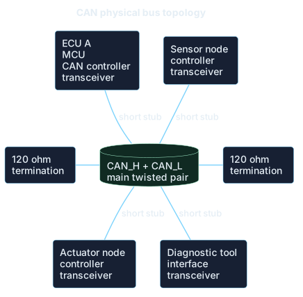
A high-speed CAN network is a shared bus: every node connects through a transceiver, while the two ends of the main line are terminated.

A high-speed CAN network normally uses two wires:

• CAN High, abbreviated as CAN_H;
• CAN Low, abbreviated as CAN_L.

These two wires are often twisted together to improve immunity against electromagnetic interference.

4. Physical Layer: CAN High, CAN Low, and Differential Transmission

CAN uses differential transmission.

This means that the receiver does not interpret the absolute voltage of a single wire, but the voltage difference between CAN_H and CAN_L.

In a simplified way:

The key point is that electromagnetic noise tends to affect both wires in a similar way. The receiver, however, reads the difference between the two signals. This makes CAN much more resistant to noise than a single-ended signal.

That said, CAN is not magically immune to errors if the network is poorly designed.

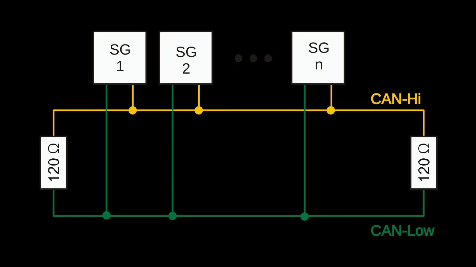
In high-speed CAN networks, the recommended topology is a main bus line with short stubs. Termination is essential: normally, two 120 ohm resistors are required, one at each end of the bus.

With two correct 120 ohm terminations at the ends, the resistance measured between CAN_H and CAN_L with the network powered off is approximately:

120 ohm || 120 ohm = 60 ohm

So, in practice:

• if we measure around 60 ohm, the terminations are probably correct;
• if we measure much more than 60 ohm, a termination may be missing;
• if we measure much less than 60 ohm, there may be too many terminations or a short circuit.

This is one of the first checks to make when a CAN network does not communicate.

5. Dominant and Recessive: The Logic of CAN

In CAN there are two fundamental states:

The CAN bus behaves like a wired-AND logic: if at least one node transmits a dominant bit, the bus becomes dominant. The bus remains recessive only if all nodes transmit recessive.

This mechanism is the foundation of two very important functions:

• message arbitration;
• error detection through bit monitoring.

A node that transmits does not just send data: it continuously reads the bus. If it transmits recessive but reads dominant, it understands that another node is forcing a dominant bit.

This is exactly what allows CAN to handle simultaneous transmissions without destroying the winning message.

6. CAN Arbitration: Priority Without Destructive Collisions

CAN is a multi-master network.

There is no single master that authorizes the other nodes to speak. Any node can start transmitting when the bus is free.

If two or more nodes start transmitting at the same time, CAN uses bit-by-bit arbitration on the identifier field.

During arbitration, each node transmits its own ID and reads the bus at the same time. Since the dominant bit wins over the recessive bit, the message with the numerically lower ID wins arbitration.

The node that loses stops transmitting and tries again later. The message that wins continues without being corrupted. This is why we call it non-destructive arbitration.

Simplified example:

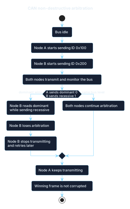
During arbitration, a node that sends recessive but reads dominant loses and stops, while the winning frame continues.

Node A wins because its ID contains a dominant bit earlier, while Node B is transmitting a recessive bit.

The practical consequence is very important: the most urgent messages must have lower IDs.

In an automotive network, messages related to braking, engine control, torque, safety, or vehicle dynamics must have higher priority than messages related to comfort, climate control, or infotainment.

7. CAN Message Formats

CAN transmits data in the form of frames.

In classic CAN there are two main formats:

The 11-bit standard frame allows 2048 theoretical identifiers.

The 29-bit extended frame allows many more identifiers and is widely used by protocols such as SAE J1939.

A common mistake is thinking that the CAN ID is the receiver address. In reality, in classic CAN, the CAN ID mainly identifies the type of message and its priority.

All nodes physically receive the frame, but only the interested ones process it.

8. Structure of a Classic CAN Data Frame

A classic CAN data frame contains several fields.

SOF - Start of Frame

This is a dominant bit that marks the beginning of a new frame. It also helps synchronize the nodes.

Arbitration Field

This field contains the CAN ID and the bits needed to distinguish standard frames, extended frames, and remote frames. It is the field used to decide which message wins if multiple nodes start transmitting at the same time.

Control Field

This field contains the DLC, meaning Data Length Code. In classic CAN, the DLC indicates how many bytes are present in the payload, from 0 to 8.

Data Field

This contains the actual data. In classic CAN, the maximum payload is 8 bytes, or 64 bits.

CRC Field

This is used to detect transmission errors. The transmitter calculates a CRC code, and the receivers verify whether the received value is consistent with the frame content.

ACK Field

The transmitter sends the ACK bit as recessive. If at least one receiver has correctly received the frame, it forces the ACK bit dominant.

This way, the transmitter knows that at least one node acknowledged the message.

EOF

This marks the end of the frame and is formed by a recessive sequence.

9. Types of CAN Frames

In classic CAN there are four main frame types:

In modern networks, the most important one is the data frame.

Remote frames are rarely used in current architectures, mainly because many higher-level protocols prefer normal request-response messages.

Also, remote frames are not supported by CAN FD.

10. Bit Timing: How Nodes Stay Synchronized

CAN does not transmit a separate clock.

All nodes must therefore synchronize on signal edges. This is why bit timing is a fundamental part of CAN configuration.

Each bit is divided into time units called time quanta. These time quanta are organized into logical segments.

The main segments are:

The sample point is especially important: it is the instant when the controller reads the bit value.

Incorrect bit timing can cause:

• intermittent errors;
• lost frames;
• frequent error frames;
• bus-off;
• unstable communication;
• problems that appear only at certain temperatures or cable lengths.

Typical parameters to configure in a CAN controller:

Examples of common bitrates:

The correct bitrate alone is not enough. The sample point, SJW, and timing segments must also be consistent with the physical bus and with the other nodes.

11. Bit Stuffing

CAN uses bit stuffing to maintain enough transitions on the bus and help synchronization.

The rule is this: after five consecutive bits of the same value, the transmitter automatically inserts one complementary bit.

So, after five consecutive dominant bits, one recessive bit is inserted. After five consecutive recessive bits, one dominant bit is inserted.

Example:

Original sequence:

00000

Transmitted sequence with stuffing:

000001

The added bit is not part of the application data. The receiver automatically removes it during reception.

If a receiver sees six consecutive equal bits in a part of the frame where bit stuffing is expected, a stuff error is generated.

Bit stuffing also has a practical consequence: the real length of a frame can vary slightly depending on the payload content, because some data generates more stuff bits than others.

12. CAN Message and CAN Signal: A Fundamental Difference

In everyday language, people often talk about "CAN signals," but technically the bus transports frames.

A signal is logical information contained inside the payload of a frame.

So:

• a CAN message is the frame identified by a CAN ID;
• a CAN signal is a variable contained in the frame data field.

Example:

A classic CAN payload contains a maximum of 8 bytes. Inside these 8 bytes, multiple signals can be encoded, each with:

• start bit;
• bit length;
• byte order;
• signedness;
• scale;
• offset;
• unit of measurement;
• valid range;
• physical value.

This distinction is one of the most important of all: the frame is the container, the signal is the interpreted information.

13. DBC: The Database That Gives Meaning to Bytes

A raw CAN log may look like this:

timestamp: 12.345678ID: 0x0CF00400DLC: 8DATA: FF FF FF 68 13 FF FF FF

Without a description of the content, these bytes are almost useless.

To decode them, we often use a DBC file, meaning a CAN database.

A DBC describes messages and signals, including information such as start bit, length, byte order, signedness, scale, and offset.

Typical DBC elements:

The conversion formula is:

physical value = raw value * factor + offset

Simplified DBC example:

BO_ 256 EngineData: 8 ECU_Engine SG_ EngineSpeed : 0|16@1+ (0.125,0) [0|8000] "rpm" ECU_Dashboard SG_ CoolantTemp : 16|8@1+ (1,-40) [-40|215] "degC" ECU_Dashboard SG_ Torque      : 24|16@1- (0.1,0) [-3200|3200] "Nm" ECU_Gateway

Interpretation:

• BO_ 256 defines a message with decimal ID 256, meaning 0x100;
• EngineData is the message name;
• 8 is the DLC;
• EngineSpeed starts at bit 0, is 16 bits long, little-endian, and unsigned;
• the physical engine speed value is raw * 0.125;
• CoolantTemp uses an offset of -40, so a raw value of 90 corresponds to 50 deg C.

This part is essential: CAN does not say by itself that a byte represents temperature, speed, or torque. The meaning comes from the database.

14. Endianness: Intel and Motorola

One of the most delicate aspects of CAN decoding is endianness.

In DBC files, we often find two formats:

Endianness determines how the bits of a multi-byte signal are ordered inside the payload.

An endianness mistake can produce completely wrong values even if the ID, scale, and offset are correct.

Example:

Payload:

10 27

If interpreted as little-endian:

0x2710 = 10000

If interpreted as big-endian:

0x1027 = 4135

The physical result can therefore change drastically.

This is one of the first things to check when a decoded value "looks plausible but does not add up."

15. Acceptance Filtering

Every CAN node physically receives all frames present on the bus, but not all frames are useful.

To avoid overloading the microcontroller, the CAN controller can use hardware acceptance filters.

A filter can accept only:

• specific IDs;
• ID ranges;
• standard IDs;
• extended IDs;
• frames matching certain masks.

Examples:

The filter does not prevent the frame from circulating on the bus. It only helps the node decide what should be passed to the application software.

So, if a message "does not arrive" in the software, it does not always mean that it does not exist on the bus. It may have been filtered at the hardware level.

16. Error Handling in CAN

CAN is very robust because it includes several error detection mechanisms.

The main errors are:

When an error is detected, a node transmits an error frame.

The message is invalidated, and the transmitter will try to retransmit it.

This automatic error handling is one of the reasons why CAN is very suitable for noisy environments and real-time applications.

17. Error Active, Error Passive, and Bus-Off

Each CAN node maintains internal error counters, typically:

• TEC, Transmit Error Counter;
• REC, Receive Error Counter.

Based on these counters, a node can be in three states:

Bus-off is an important protection mechanism: if a faulty node keeps generating errors, the protocol can isolate it to prevent the whole network from becoming unusable.

Typical causes of bus-off:

• wrong bitrate;
• faulty wiring;
• faulty transceiver;
• missing ACK;
• wrong terminations;
• electrical noise;
• no common ground;
• software bug causing continuous transmission of incorrect frames.

In practice, when a node goes bus-off, we should not only look at the firmware. We also need to check wiring, terminations, bitrate, and the presence of other active nodes on the bus.

18. Message Frequency and Bus Load

In a CAN network, messages can be:

• periodic;
• event-driven;
• request-based;
• diagnostic;
• cyclic with timeout.

Example:

Bus load indicates how much of the network capacity is occupied by frames.

A CAN network with excessive bus load can introduce delays, worsen the latency of lower-priority messages, and make diagnostics more difficult.

During design, we need to consider:

• average frame length;
• bitrate;
• message frequency;
• priority;
• number of nodes;
• diagnostic traffic;
• free margin for future extensions.

A cautious rule is to avoid designing networks that constantly run close to 100% load. In real applications, we need margin for retransmissions, diagnostics, and abnormal conditions.

A network that works in ideal conditions but has no margin can become unstable as soon as traffic increases or an error appears.

19. Higher-Level Protocols: CAN as a Base, Not a Complete Application

CAN defines frame transport, but it does not define the application meaning of the data.

This is why higher-level protocols exist.

The most important ones are:

So CAN is the base. Above it, each sector builds its own way of representing data, diagnostics, configurations, and commands.

20. OBD2 over CAN

OBD2, meaning On-Board Diagnostics, is the standard diagnostic system used in vehicles to access parameters and fault codes mainly related to emissions and engine operation.

OBD2 uses the concept of PID, or Parameter ID.

A tester sends a request, and the ECU replies with the requested data.

Conceptual example:

OBD2 is useful, but limited. It exposes only part of the data available in the vehicle.

More detailed data is often available through UDS or proprietary protocols.

21. UDS and ISO-TP

UDS, meaning Unified Diagnostic Services, is a diagnostic protocol used for advanced diagnostics, testing, data reading, parameter writing, ECU reset, and firmware updates.

UDS often runs over CAN using ISO-TP, meaning ISO 15765-2.

The reason is simple: classic CAN can carry only 8 bytes per frame, while many diagnostic responses are longer.

ISO-TP solves this problem by segmenting larger messages into multiple CAN frames.

ISO-TP uses several frame types:

UDS example:

VIN read request:

22 F1 90

Where:

• 0x22 is the UDS ReadDataByIdentifier service;
• 0xF190 is a DID commonly used for the VIN.

A VIN response is longer than 8 bytes, so it is segmented through ISO-TP.

This is a perfect example of the relationship between layers: CAN transports the frames, ISO-TP manages multi-frame transport, and UDS defines the diagnostic meaning of the request.

22. SAE J1939

SAE J1939 is a higher-level protocol based on CAN, widely used in heavy-duty vehicles, trucks, buses, agricultural machines, industrial engines, and off-highway vehicles.

J1939 uses extended 29-bit CAN identifiers.

In the J1939 world, a central concept is the PGN, meaning Parameter Group Number. The PGN is a subset of the extended 29-bit CAN ID and represents the logical identifier of the message.

Simplified structure of the J1939 ID:

Key concepts:

PGN examples:

In the J1939 world, the DBC is often built around PGN/SPN rather than a single physical ID.

This makes J1939 very structured and suitable for complex vehicles where the engine, transmission, brakes, implements, and external modules must communicate in a standardized way.

23. CANopen

CANopen is a higher-level protocol mainly used in industrial automation, motion control, robotics, inverters, intelligent sensors, and machines.

Main concepts:

CANopen adds a complete application structure on top of CAN.

While CAN defines how to transmit frames, CANopen defines how to represent objects, parameters, states, and cyclic data.

It is widely used when a network must be organized, with configurable devices and standardized behavior.

24. CAN FD: The Evolution of Classic CAN

Classic CAN has two important limits:

• maximum payload of 8 bytes;
• maximum nominal speed typically up to 1 Mbit/s.

CAN FD, meaning CAN Flexible Data-rate, was introduced to overcome these limits.

CAN FD allows two different bitrates:

• one during the arbitration phase;
• a higher one during the data phase.

It also increases the maximum payload to 64 bytes.

Main differences:

Important CAN FD fields:

BRS, Bit Rate Switch, allows the data phase to be transmitted at a higher speed than the arbitration phase.

CAN FD is useful for:

• ECU flashing;
• faster diagnostics;
• high-volume data logging;
• sensors with larger payloads;
• modern automotive networks;
• reducing overhead per useful byte.

In practice, CAN FD keeps many ideas from classic CAN, but increases capacity and efficiency.

25. CAN XL: The Next Evolution

CAN XL, meaning CAN eXtended data-field Length, is the next evolution after classic CAN and CAN FD.

CAN XL supports data fields from 1 byte up to 2048 bytes.

Comparison:

CAN XL also introduces a clearer distinction between priority and acceptance.

In classic CAN and CAN FD, the ID is used both for arbitration and identification. In CAN XL, these functions are separated using an 11-bit priority ID and a 32-bit acceptance field.

CAN XL is designed for cases where we need:

• very large payloads;
• higher efficiency;
• integration with modern architectures;
• transport of complex data;
• possible connection with IP networks;
• more efficient software updates.

CAN XL does not immediately replace classic CAN or CAN FD, but expands the CAN family toward more demanding applications.

26. CAN Logging: From Raw Frame to Physical Data

To analyze a CAN network, we record traffic using tools such as:

• CAN-USB interfaces;
• standalone data loggers;
• Vector tools;
• Kvaser;
• Peak;
• CSS Electronics;
• oscilloscopes;
• CAN-Ethernet gateways;
• SocketCAN software;
• sniffing and reverse engineering tools.

A raw log typically contains:

Example in candump format:

can0  100   [8]  10 27 5A 00 80 01 00 FFcan0  200   [8]  34 12 00 00 01 00 AA 55

Decoding through a DBC:

EngineSpeed = 1250 rpmCoolantTemp = 50 deg CBrakePressed = falseVehicleSpeed = 86.5 km/h

The correct analysis flow is:

• identify bitrate and frame format;
• record the traffic;
• distinguish standard and extended frames;
• apply the correct DBC;
• validate scale, offset, and endianness;
• check frequencies and timeouts;
• correlate signals with real events;
• check error frames and bus load.

This is the difference between looking at bytes and actually performing CAN analysis.

27. Reverse Engineering CAN Signals

When an official DBC is not available, reverse engineering may be necessary.

The typical method is:

Example for finding the brake signal:

• record traffic with the brake released;
• press the brake;
• compare the payloads;
• look for bits changing from 0 to 1;
• verify repeatability;
• create the signal in the DBC.

Example for finding vehicle speed:

• record with the vehicle stopped;
• record at 20, 40, and 60 km/h;
• look for values that increase linearly;
• estimate factor and offset;
• validate with GPS or OBD2.

This requires a lot of caution. In modern vehicles, reverse engineering can have legal, safety, and warranty implications.

It should be done only in controlled environments and without transmitting active frames on critical networks, unless we know exactly what we are doing.

28. Practical Diagnostics of a CAN Network

When a CAN network does not work correctly, we need to analyze both the physical layer and the logical layer.

Physical Checks

Logical Checks

Oscilloscope

With an oscilloscope we can observe:

• differential amplitude;
• edges that are too slow;
• reflections;
• noise;
• overshoot;
• distortion;
• symmetry between CAN_H and CAN_L.

A logic analyzer or a CAN interface can tell us that there are errors. An oscilloscope helps us understand whether the cause is physical.

This difference is fundamental: the software may look like the problem, but the physical bus may tell a different story.

29. CAN Cybersecurity

Classic CAN was designed for closed and controlled networks.

It does not natively include:

• sender authentication;
• encryption;
• permission control;
• protection against replay attacks;
• strong protection against spoofing;
• automatic isolation between functional domains.

This means that a node with access to the bus can potentially listen to or inject frames.

In modern vehicles, the issue is mitigated through:

• gateways;
• segmentation;
• automotive firewalls;
• secure diagnostics;
• intrusion detection systems;
• application-level controls.

Typical risks:

Security cannot be solved only at the CAN level. It must be designed at the vehicle or machine architecture level.

CAN is robust as a communication protocol, but it is not secure by default from a cybersecurity perspective.

30. Common Mistakes to Avoid

The most common mistakes in CAN design or analysis are:

• confusing the CAN ID with a receiver address;
• thinking that CAN directly transports physical values;
• using the wrong DBC;
• ignoring endianness and signedness;
• configuring the wrong bitrate;
• forgetting terminations;
• using too many terminations;
• creating stubs that are too long;
• transmitting frames on a real network without knowing their effect;
• not considering bus load and priority;
• not distinguishing classic CAN, CAN FD, and CAN XL;
• using an interface that does not support CAN FD on a CAN FD network;
• ignoring error counters and bus-off state;
• analyzing only the software without checking the physical layer.

Many CAN problems start exactly here: we look at the log but do not check the bus. Or we check the wiring but ignore the DBC. We always need a complete view.

31. Complete Example: From Frame to Physical Value

Let's look at a complete example.

Received frame:

ID: 0x100DLC: 8DATA: 10 27 82 00 2C 01 00 FF

Simplified DBC:

BO_ 256 EngineData: 8 ECU_Engine SG_ EngineSpeed : 0|16@1+ (0.125,0) [0|8000] "rpm" ECU_Dashboard SG_ CoolantTemp : 16|8@1+ (1,-40) [-40|215] "degC" ECU_Dashboard SG_ PedalPos    : 32|8@1+ (0.4,0) [0|100] "%" ECU_Dashboard

EngineSpeed

Bytes 0-1:

10 27

Little-endian:

0x2710 = 10000

Scale:

10000 * 0.125 = 1250 rpm

CoolantTemp

Byte 2:

0x82 = 130

Scale and offset:

130 * 1 - 40 = 90 deg C

PedalPos

Byte 4:

0x2C = 44

Scale:

44 * 0.4 = 17.6 %

Final result:

This example shows the key point: the frame contains only bytes. The DBC is what allows us to transform them into engineering data.

Without the DBC, 10 27 82 00 2C 01 00 FF remains only a sequence of bytes. With the correct DBC, it becomes useful information.

32. Final Comparison: CAN, CAN FD, and CAN XL

Classic CAN is still widely used for simple, robust, and deterministic communication.

CAN FD is now the better choice when more data and higher speed are needed.

CAN XL represents the most recent evolution for architectures that require much larger payloads and better integration with modern networks.

We should not think of them as three technologies competing directly with each other. They are three evolutionary levels of the same family, to be chosen according to the application.

33. Conclusion

The CAN protocol is one of the pillars of embedded and automotive communication because it combines simplicity, robustness, deterministic priority, and advanced error handling.

To really understand it, we need to separate three levels.

• Physical layer: cables, CAN_H, CAN_L, terminations, transceivers, differential levels, topology, bus length, and signal quality.
• Data link layer: frames, IDs, arbitration, bit stuffing, CRC, ACK, error frames, error counters, and bus-off.
• Application layer: data meaning, signals, DBC, diagnostics, OBD2, UDS, ISO-TP, J1939, CANopen, and proprietary protocols.

CAN does not directly transmit "speed," "temperature," or "torque." It transmits binary frames.

The meaning of those frames comes from the way bits are mapped into signals, scaled, and interpreted.

For this reason, in professional analysis, knowing how to read a CAN ID is not enough. We need to understand the physical layer, frame structure, timing, DBC, errors, higher-level protocols, and application context.

In short, CAN is a technology that looks simple from the outside, but is extremely refined underneath.

Its effectiveness comes from the combination of differential transmission, non-destructive arbitration, deterministic priority, error detection, and application flexibility.

And this combination is exactly why CAN is still essential today in vehicles, industrial machines, embedded systems, and modern devices that need to communicate reliably.

Last updated 2026-07-06.
Article source content/blog/can_protocol.